The choice - 1 (Intro)

2011 Jul 22

[ Get the code at github ]

A programming language is low level when its programs require attention to the irrelevant. Quote: – Alan J. Perlis

It’s not only that physicists can’t program (we rarely use version control, we don’t plan, we don’t test… I suppose most labs score zero on The Joel Test). It is that we program, we program a lot and we still mostly use Fortran!

Now I’m not implying that Fortran is not a good language. Fortran is just fine. What I’m saying is that Fortran is a very bad choice for non-programmers who do a lot of programming.

Over the years some have turned to other languages like C, C++ and Matlab. Some, perhaps more enlightened, have even turned to Python. Naturally, I, too, turned to other languages and soon began wondering about what else might be out there (language-wise) to help a poor physicist do his job.

Could there be a language that won’t break everything apart just because a number is consider “special”? (What’s a float or a double? Why do I care?) Could there be one that implements a few-lines-of-equations-model in a few lines of code? One that will help me in my work not make the problem just … different?

I’ve been googling and poking around on stackoverflow and programmers.SE for some answers but nothing particularly interesting came up. It, thus, seems that I have to try them all.

“Rules”: no extra packages; idiomatic code for each language; efficiency is not so much of an issue; extendable code

The system

I’ll be solving, as an example, the following 2D system of ordinary differential equations:

$$ \begin{aligned} \frac{df_1(x)}{dx} =& 1 - f_2(x)\\ \frac{df_2(x)}{dx} =& f_1(x) - x \end{aligned} $$

with initial conditions:

$$\begin{aligned} x_0 &= 0\\ f_1(x_0) &= 1\\ f_2(x_0) &= 0 \end{aligned}$$

in the range $$[0, 3]$$

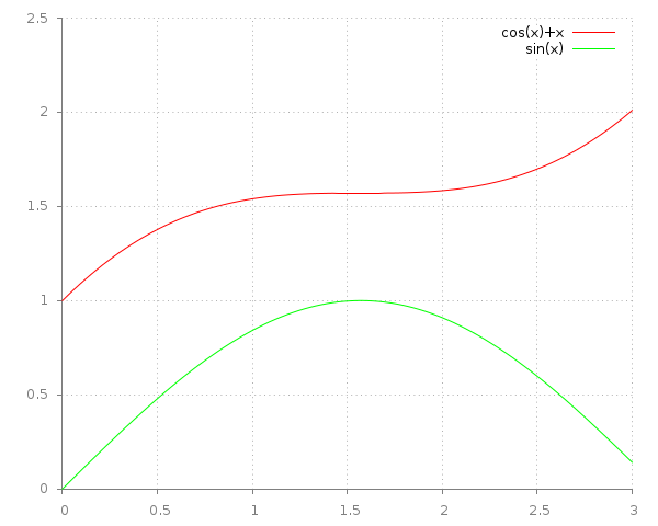
The exact solution is $$\begin{aligned} f_1(x)&=\cos{x}+x\\ f_2(x)&=\sin{x}\end{aligned}$$

solution

To numerically solve the system we treat the function values $$f_i(x)$$ as parameters of the differential functions:

$$\begin{aligned} F_1(x,y_1,y_2) &= \frac{df_1(x,y_1,y_2)}{dx} =& 1 - y_2\\ F_2(x,y_1,y_2) &= \frac{df_2(x,y_1,y_2)}{dx} =& y_1 - x \end{aligned}$$

We will end up with a list of $y_{i,0},\ldots,y_{i,n}$ values that will represent an approximation of the values $f_i(x_k),\, x_k = x + k\cdot\delta x$.

The method: Runge Kutta-4

Runge Kutta method iterates from a current known value of $$f(x)$$ to the “next” value at $$x+\delta x$$. So, knowing $$f(x_0)$$ and choosing a small step $$\delta x$$ the method gives us $$f(x_0 + \delta x)$$ by calculating a “correction” to $$f(x_0)$$.

We thus have: $$ f(x_0 + \delta x) = f(x_0) + \Delta()$$ where the correction $$\Delta()$$ depends on $$\delta x, x_0, f(x_0), f\prime(x,y)$$ and is given by:

$$ \Delta(\delta x, x_0, f(x_0), f\prime(x,y)) = \frac{1}{6}\delta x (a + 2b + 2c + d) $$

where

$$\begin{aligned} a =& f\prime(x_0, f(x_0))\
b = & f\prime(x_0 + \frac{1}{2}\delta x, f(x_0) + \frac{1}{2}a\delta x)\
c = & f\prime(x_0 + \frac{1}{2}\delta x, f(x_0) + \frac{1}{2}b\delta x)\
d = & f\prime(x_0 + \delta x, f(x_0) + c\delta x)\
\end{aligned}$$

We feed $$\Delta()$$ with the initial known values.

In many dimensions

To apply RK4 to a system of ODEs

for each set of equations $$F_i = f_i\prime(x_0, y_1, \ldots, y_n)$$ we have a different set of parameters $$a_i, b_i, c_i, d_i$$ and a correction function $$f_i(x_0 + \delta x) = f_i(x_0) + \Delta(\delta x, a_i,b_i,c_i,d_i) $$

$$\begin{aligned} a_i &= F_i(x_0 ,& y_1,& \ldots ,& y_n) \\ b_i &= F_i(x_0+\frac{1}{2}\delta x ,& y_1 + \frac{1}{2}a_1\delta x ,& \ldots ,& y_n + \frac{1}{2}a_n\delta x)\\ c_i &= F_i(x_0+\frac{1}{2}\delta x ,& y_1 + \frac{1}{2}b_1\delta x ,& \ldots ,& y_n + \frac{1}{2}b_n\delta x)\\ d_i &= F_i(x_0+\delta x ,& y_1 + c_1\delta x ,& \ldots ,& y_n + c_n\delta x)\\ \end{aligned}$$

$$ \Delta() = \frac{1}{6}\delta x (a_i + 2 b_i + 2 c_i + d) $$

$$ f_i(x_0 + \delta x) = f_i(x_0) + \Delta(\delta x, a_i,b_i,c_i,d_i) $$

The Code

I’ll use a C implementation as a reference.

C (reference)

Adapted from numerical recipes in C:

<{{static/src/the-choice-1-intro/rk4.c}}

for example: <{{static/src/the-choice-1-intro/rk4_ex.c}}

Coming up: J, LISP, R, Fortran, Python, Haskell, Pari/GP, maxima.